Flu Analysis Model Evaluation

Loading packages

library(tidyverse)

── Attaching packages ─────────────────────────────────────── tidyverse 1.3.2 ──
✔ ggplot2 3.4.0      ✔ purrr   1.0.1 
✔ tibble  3.1.8      ✔ dplyr   1.0.10
✔ tidyr   1.2.1      ✔ stringr 1.5.0 
✔ readr   2.1.3      ✔ forcats 0.5.2 
── Conflicts ────────────────────────────────────────── tidyverse_conflicts() ──
✖ dplyr::filter() masks stats::filter()
✖ dplyr::lag()    masks stats::lag()

library(tidymodels)

── Attaching packages ────────────────────────────────────── tidymodels 1.0.0 ──
✔ broom        1.0.2     ✔ rsample      1.1.1
✔ dials        1.1.0     ✔ tune         1.0.1
✔ infer        1.0.4     ✔ workflows    1.1.2
✔ modeldata    1.0.1     ✔ workflowsets 1.0.0
✔ parsnip      1.0.3     ✔ yardstick    1.1.0
✔ recipes      1.0.4     
── Conflicts ───────────────────────────────────────── tidymodels_conflicts() ──
✖ scales::discard() masks purrr::discard()
✖ dplyr::filter()   masks stats::filter()
✖ recipes::fixed()  masks stringr::fixed()
✖ dplyr::lag()      masks stats::lag()
✖ yardstick::spec() masks readr::spec()
✖ recipes::step()   masks stats::step()
• Learn how to get started at https://www.tidymodels.org/start/

library(skimr)

Load Data

#load in data set
fludata<-readRDS("../data/flurevised.rds")

Data Splitting

set.seed(222)
data_split <- initial_split(fludata, prop=3/4)
train_data <- training(data_split)
test_data  <- testing(data_split)

Create Recipe

#create recipe
flu_rec <- 
  recipe(Nausea ~ ., data = train_data) 
#model specification
lr_mod <- 
  logistic_reg() %>% 
  set_engine("glm")
#workflow
flu_wflow <- 
  workflow() %>% 
  add_model(lr_mod) %>% 
  add_recipe(flu_rec)
flu_wflow

══ Workflow ════════════════════════════════════════════════════════════════════
Preprocessor: Recipe
Model: logistic_reg()

── Preprocessor ────────────────────────────────────────────────────────────────
0 Recipe Steps

── Model ───────────────────────────────────────────────────────────────────────
Logistic Regression Model Specification (classification)

Computational engine: glm 

#create the fit from the established workflow
flu_fit <- 
  flu_wflow %>% 
  fit(data = train_data)
#check prediction to evaluate test data
predict(flu_fit, test_data)

Warning in predict.lm(object, newdata, se.fit, scale = 1, type = if (type == :
prediction from a rank-deficient fit may be misleading

# A tibble: 183 × 1
   .pred_class
   <fct>      
 1 No         
 2 No         
 3 No         
 4 No         
 5 No         
 6 Yes        
 7 Yes        
 8 No         
 9 No         
10 Yes        
# … with 173 more rows

Evaluate Performance

#Augment to return probabilities rather than yes or no
flu_aug <- 
  augment(flu_fit, test_data)

Warning in predict.lm(object, newdata, se.fit, scale = 1, type = if (type == :
prediction from a rank-deficient fit may be misleading

Warning in predict.lm(object, newdata, se.fit, scale = 1, type = if (type == :
prediction from a rank-deficient fit may be misleading

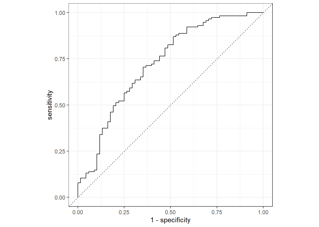
#Use roc_curve to evaluate model
flu_aug %>% 
  roc_curve(truth = Nausea, .pred_No) %>% 
  autoplot()

#Use roc_aug to quantify area under roc-curve
flu_aug %>% 
  roc_auc(truth = Nausea, .pred_No)

# A tibble: 1 × 3
  .metric .estimator .estimate
  <chr>   <chr>          <dbl>
1 roc_auc binary         0.724

According to the ROC metric, this model is useful as it is over 0.7 at 0.724.

Make model with Main Predictor of Interest

#recipe
flu_runnynose <- 
  recipe(Nausea ~ RunnyNose, data = train_data) 
#workflow
flu_wflow_runnynose <- 
  workflow() %>% 
  add_model(lr_mod) %>% 
  add_recipe(flu_runnynose)
#create fit
flu_runnynose_fit <- 
  flu_wflow_runnynose %>% 
  fit(data = train_data)

Evaluate Performance

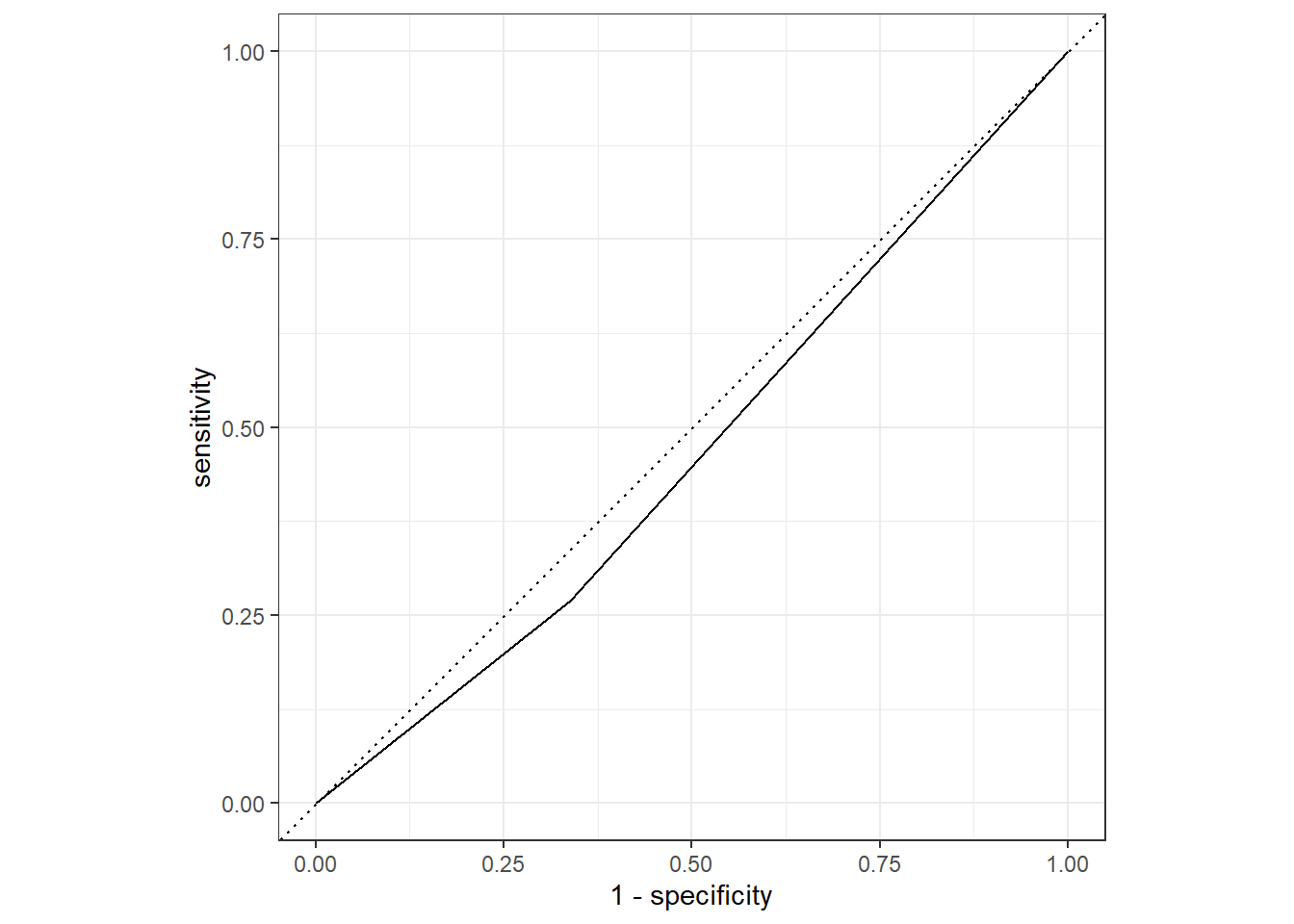
#Augment to return probabilities rather than yes or no
flu_runnynose_aug <- 
  augment(flu_runnynose_fit, test_data)
#Use roc_curve to evaluate model
flu_runnynose_aug %>% 
  roc_curve(truth = Nausea, .pred_No) %>% 
  autoplot()

#Use roc_aug to quantify area under roc-curve
flu_runnynose_aug %>% 
  roc_auc(truth = Nausea, .pred_No)

# A tibble: 1 × 3
  .metric .estimator .estimate
  <chr>   <chr>          <dbl>
1 roc_auc binary         0.466

Since the ROC is estimated to be 0.466, it is not a well performing model according to this metric.

Kelly Hatfield’s Additions

Model with all predictors

#create the recipe and workflow
flu_rec_lin <- 
  recipe(BodyTemp ~ ., data = train_data) 
#model specification
lin_mod <- 
  linear_reg() %>% 
  set_engine("lm")
#workflow
flu_wflow_lin <- 
  workflow() %>% 
  add_model(lin_mod) %>% 
  add_recipe(flu_rec_lin)
flu_wflow_lin

══ Workflow ════════════════════════════════════════════════════════════════════
Preprocessor: Recipe
Model: linear_reg()

── Preprocessor ────────────────────────────────────────────────────────────────
0 Recipe Steps

── Model ───────────────────────────────────────────────────────────────────────
Linear Regression Model Specification (regression)

Computational engine: lm 

#create the fit from the established workflow
flu_fit_lin <- 
  flu_wflow_lin %>% 
  fit(data = train_data)
#check prediction to evaluate test data
predict(flu_fit_lin, test_data)

Warning in predict.lm(object = object$fit, newdata = new_data, type =
"response"): prediction from a rank-deficient fit may be misleading

# A tibble: 183 × 1
   .pred
   <dbl>
 1  99.3
 2  99.0
 3  99.7
 4  98.7
 5  99.0
 6  99.5
 7  99.3
 8  98.9
 9  99.6
10  98.8
# … with 173 more rows

#Augment to return probabilities 
flu_aug_lin <- 
  augment(flu_fit_lin, test_data)

Warning in predict.lm(object = object$fit, newdata = new_data, type =
"response"): prediction from a rank-deficient fit may be misleading

#Calculate mse
#train model

flu_aug_train_lin <- 
  augment(flu_fit_lin, train_data)

Warning in predict.lm(object = object$fit, newdata = new_data, type =
"response"): prediction from a rank-deficient fit may be misleading

#RSME train
yardstick::rmse(flu_aug_train_lin, BodyTemp, .pred)

# A tibble: 1 × 3
  .metric .estimator .estimate
  <chr>   <chr>          <dbl>
1 rmse    standard        1.11

#RSME test

yardstick::rmse(flu_aug_lin, BodyTemp, .pred)

# A tibble: 1 × 3
  .metric .estimator .estimate
  <chr>   <chr>          <dbl>
1 rmse    standard        1.15

We see that the training data performed a bit better with our RMSE estimated to be 1.11 versus with the tested data at 1.15, but similar results

Model with 1 predictor

#create the recipe and workflow
flu_rec_lin <- 
  recipe(BodyTemp ~ RunnyNose, data = train_data) 
#model specification
lin_mod <- 
  linear_reg() %>% 
  set_engine("lm")
#workflow
flu_wflow_lin <- 
  workflow() %>% 
  add_model(lin_mod) %>% 
  add_recipe(flu_rec_lin)
flu_wflow_lin

══ Workflow ════════════════════════════════════════════════════════════════════
Preprocessor: Recipe
Model: linear_reg()

── Preprocessor ────────────────────────────────────────────────────────────────
0 Recipe Steps

── Model ───────────────────────────────────────────────────────────────────────
Linear Regression Model Specification (regression)

Computational engine: lm 

#create the fit from the established workflow
flu_fit_lin <- 
  flu_wflow_lin %>% 
  fit(data = train_data)
#check prediction to evaluate test data
predict(flu_fit_lin, test_data)

# A tibble: 183 × 1
   .pred
   <dbl>
 1  99.1
 2  98.9
 3  98.9
 4  98.9
 5  99.1
 6  99.1
 7  98.9
 8  99.1
 9  99.1
10  99.1
# … with 173 more rows

#Augment to return probabilities 
flu_aug_lin <- 
  augment(flu_fit_lin, test_data)

#Calculate mse
#train model

flu_aug_train_lin <- 
  augment(flu_fit_lin, train_data)
#RSME train
yardstick::rmse(flu_aug_train_lin, BodyTemp, .pred)

# A tibble: 1 × 3
  .metric .estimator .estimate
  <chr>   <chr>          <dbl>
1 rmse    standard        1.21

#RSME test

yardstick::rmse(flu_aug_lin, BodyTemp, .pred)

# A tibble: 1 × 3
  .metric .estimator .estimate
  <chr>   <chr>          <dbl>
1 rmse    standard        1.13

We see that the training data performed a bit better with our RMSE estimated to be 1.21 versus with the tested data at 1.13, but similar results