#look at help file for gapminder datahelp(gapminder)
starting httpd help server ... done
#get an overview of the structure of gapminder datastr(gapminder)
'data.frame':   10545 obs. of  9 variables:
 $ country         : Factor w/ 185 levels "Albania","Algeria",..: 1 2 3 4 5 6 7 8 9 10 ...
 $ year            : int  1960 1960 1960 1960 1960 1960 1960 1960 1960 1960 ...
 $ infant_mortality: num  115.4 148.2 208 NA 59.9 ...
 $ life_expectancy : num  62.9 47.5 36 63 65.4 ...
 $ fertility       : num  6.19 7.65 7.32 4.43 3.11 4.55 4.82 3.45 2.7 5.57 ...
 $ population      : num  1636054 11124892 5270844 54681 20619075 ...
 $ gdp             : num  NA 1.38e+10 NA NA 1.08e+11 ...
 $ continent       : Factor w/ 5 levels "Africa","Americas",..: 4 1 1 2 2 3 2 5 4 3 ...
 $ region          : Factor w/ 22 levels "Australia and New Zealand",..: 19 11 10 2 15 21 2 1 22 21 ...
#get a summary of datasummary(gapminder)
                country           year      infant_mortality life_expectancy
 Albania            :   57   Min.   :1960   Min.   :  1.50   Min.   :13.20
 Algeria            :   57   1st Qu.:1974   1st Qu.: 16.00   1st Qu.:57.50
 Angola             :   57   Median :1988   Median : 41.50   Median :67.54
 Antigua and Barbuda:   57   Mean   :1988   Mean   : 55.31   Mean   :64.81
 Argentina          :   57   3rd Qu.:2002   3rd Qu.: 85.10   3rd Qu.:73.00
 Armenia            :   57   Max.   :2016   Max.   :276.90   Max.   :83.90
 (Other)            :10203                  NA's   :1453
   fertility       population             gdp               continent
 Min.   :0.840   Min.   :3.124e+04   Min.   :4.040e+07   Africa  :2907
 1st Qu.:2.200   1st Qu.:1.333e+06   1st Qu.:1.846e+09   Americas:2052
 Median :3.750   Median :5.009e+06   Median :7.794e+09   Asia    :2679
 Mean   :4.084   Mean   :2.701e+07   Mean   :1.480e+11   Europe  :2223
 3rd Qu.:6.000   3rd Qu.:1.523e+07   3rd Qu.:5.540e+10   Oceania : 684
 Max.   :9.220   Max.   :1.376e+09   Max.   :1.174e+13
 NA's   :187     NA's   :185         NA's   :2972
             region
 Western Asia   :1026
 Eastern Africa : 912
 Western Africa : 912
 Caribbean      : 741
 South America  : 684
 Southern Europe: 684
 (Other)        :5586
#determine the type of object gapminder isclass(gapminder)
[1] "data.frame"
##Processing Data
#filter gapminder data for only countries in the continent of Africa and assign to africadataafricadata <-filter(gapminder, continent=="Africa")#verify structure and summary of africa data has correct number of observationsstr(africadata)
'data.frame':   2907 obs. of  9 variables:
 $ country         : Factor w/ 185 levels "Albania","Algeria",..: 2 3 18 22 26 27 29 31 32 33 ...
 $ year            : int  1960 1960 1960 1960 1960 1960 1960 1960 1960 1960 ...
 $ infant_mortality: num  148 208 187 116 161 ...
 $ life_expectancy : num  47.5 36 38.3 50.3 35.2 ...
 $ fertility       : num  7.65 7.32 6.28 6.62 6.29 6.95 5.65 6.89 5.84 6.25 ...
 $ population      : num  11124892 5270844 2431620 524029 4829291 ...
 $ gdp             : num  1.38e+10 NA 6.22e+08 1.24e+08 5.97e+08 ...
 $ continent       : Factor w/ 5 levels "Africa","Americas",..: 1 1 1 1 1 1 1 1 1 1 ...
 $ region          : Factor w/ 22 levels "Australia and New Zealand",..: 11 10 20 17 20 5 10 20 10 10 ...
summary(africadata)
         country          year      infant_mortality life_expectancy
 Algeria     :  57   Min.   :1960   Min.   : 11.40   Min.   :13.20
 Angola      :  57   1st Qu.:1974   1st Qu.: 62.20   1st Qu.:48.23
 Benin       :  57   Median :1988   Median : 93.40   Median :53.98
 Botswana    :  57   Mean   :1988   Mean   : 95.12   Mean   :54.38
 Burkina Faso:  57   3rd Qu.:2002   3rd Qu.:124.70   3rd Qu.:60.10
 Burundi     :  57   Max.   :2016   Max.   :237.40   Max.   :77.60
 (Other)     :2565                  NA's   :226
   fertility       population             gdp               continent
 Min.   :1.500   Min.   :    41538   Min.   :4.659e+07   Africa  :2907
 1st Qu.:5.160   1st Qu.:  1605232   1st Qu.:8.373e+08   Americas:   0
 Median :6.160   Median :  5570982   Median :2.448e+09   Asia    :   0
 Mean   :5.851   Mean   : 12235961   Mean   :9.346e+09   Europe  :   0
 3rd Qu.:6.860   3rd Qu.: 13888152   3rd Qu.:6.552e+09   Oceania :   0
 Max.   :8.450   Max.   :182201962   Max.   :1.935e+11
 NA's   :51      NA's   :51          NA's   :637
                       region
 Eastern Africa           :912
 Western Africa           :912
 Middle Africa            :456
 Northern Africa          :342
 Southern Africa          :285
 Australia and New Zealand:  0
 (Other)                  :  0
#create object with infant_mortality and life_expectancy out of africadatainfandlife <- africadata %>%select(infant_mortality, life_expectancy)#create object with population and life expectancy out of africadatapopandlife <- africadata %>%select(population, life_expectancy)#check structure and summary of both objects popandlife and infandlifestr(popandlife)
'data.frame':   2907 obs. of  2 variables:
 $ population     : num  11124892 5270844 2431620 524029 4829291 ...
 $ life_expectancy: num  47.5 36 38.3 50.3 35.2 ...
summary(popandlife)
   population        life_expectancy
 Min.   :    41538   Min.   :13.20
 1st Qu.:  1605232   1st Qu.:48.23
 Median :  5570982   Median :53.98
 Mean   : 12235961   Mean   :54.38
 3rd Qu.: 13888152   3rd Qu.:60.10
 Max.   :182201962   Max.   :77.60
 NA's   :51
str(infandlife)
'data.frame':   2907 obs. of  2 variables:
 $ infant_mortality: num  148 208 187 116 161 ...
 $ life_expectancy : num  47.5 36 38.3 50.3 35.2 ...
summary(infandlife)
 infant_mortality life_expectancy
 Min.   : 11.40   Min.   :13.20
 1st Qu.: 62.20   1st Qu.:48.23
 Median : 93.40   Median :53.98
 Mean   : 95.12   Mean   :54.38
 3rd Qu.:124.70   3rd Qu.:60.10
 Max.   :237.40   Max.   :77.60
 NA's   :226
##Initial Plotting
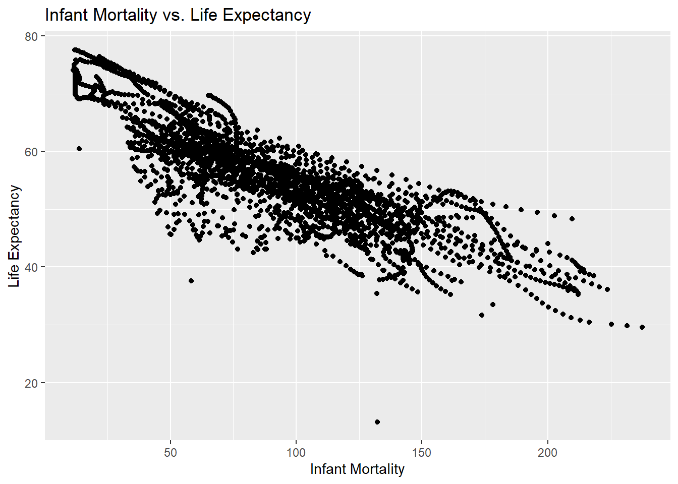
#create a scatterplot of infant_mortality and life_expectancyggplot(data=infandlife, aes(x=infant_mortality, y=life_expectancy))+geom_point()+xlab("Infant Mortality")+ylab("Life Expectancy")+labs(title="Infant Mortality vs. Life Expectancy")
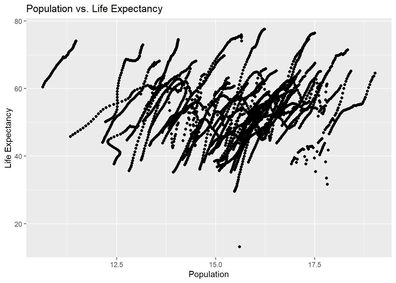
#create a scatterplot of population and life expectancy with population on the log scaleggplot(data=popandlife, aes(x=log(population), y=life_expectancy))+geom_point()+xlab("Population")+ylab("Life Expectancy")+labs(title="Population vs. Life Expectancy")
#group the africadata by year and filter missing data on infant mortality by yearafricadata %>%select(year, infant_mortality) %>%group_by(year) %>%filter(is.na(infant_mortality)) %>%count()
# A tibble: 23 × 2
# Groups:   year [23]
    year     n
   <int> <int>
 1  1960    10
 2  1961    17
 3  1962    16
 4  1963    16
 5  1964    15
 6  1965    14
 7  1966    13
 8  1967    11
 9  1968    11
10  1969     7
# … with 13 more rows
#create a new object filtering africadata for only the year 2000africa2000 <-filter(africadata, year==2000)#confirm new object africa2000 has correct number of observationsstr(africa2000)
'data.frame':   51 obs. of  9 variables:
 $ country         : Factor w/ 185 levels "Albania","Algeria",..: 2 3 18 22 26 27 29 31 32 33 ...
 $ year            : int  2000 2000 2000 2000 2000 2000 2000 2000 2000 2000 ...
 $ infant_mortality: num  33.9 128.3 89.3 52.4 96.2 ...
 $ life_expectancy : num  73.3 52.3 57.2 47.6 52.6 46.7 54.3 68.4 45.3 51.5 ...
 $ fertility       : num  2.51 6.84 5.98 3.41 6.59 7.06 5.62 3.7 5.45 7.35 ...
 $ population      : num  31183658 15058638 6949366 1736579 11607944 ...
 $ gdp             : num  5.48e+10 9.13e+09 2.25e+09 5.63e+09 2.61e+09 ...
 $ continent       : Factor w/ 5 levels "Africa","Americas",..: 1 1 1 1 1 1 1 1 1 1 ...
 $ region          : Factor w/ 22 levels "Australia and New Zealand",..: 11 10 20 17 20 5 10 20 10 10 ...
summary(africa2000)
         country        year      infant_mortality life_expectancy
 Algeria     : 1   Min.   :2000   Min.   : 12.30   Min.   :37.60
 Angola      : 1   1st Qu.:2000   1st Qu.: 60.80   1st Qu.:51.75
 Benin       : 1   Median :2000   Median : 80.30   Median :54.30
 Botswana    : 1   Mean   :2000   Mean   : 78.93   Mean   :56.36
 Burkina Faso: 1   3rd Qu.:2000   3rd Qu.:103.30   3rd Qu.:60.00
 Burundi     : 1   Max.   :2000   Max.   :143.30   Max.   :75.00
 (Other)     :45
   fertility       population             gdp               continent
 Min.   :1.990   Min.   :    81154   Min.   :2.019e+08   Africa  :51
 1st Qu.:4.150   1st Qu.:  2304687   1st Qu.:1.274e+09   Americas: 0
 Median :5.550   Median :  8799165   Median :3.238e+09   Asia    : 0
 Mean   :5.156   Mean   : 15659800   Mean   :1.155e+10   Europe  : 0
 3rd Qu.:5.960   3rd Qu.: 17391242   3rd Qu.:8.654e+09   Oceania : 0
 Max.   :7.730   Max.   :122876723   Max.   :1.329e+11

                       region
 Eastern Africa           :16
 Western Africa           :16
 Middle Africa            : 8
 Northern Africa          : 6
 Southern Africa          : 5
 Australia and New Zealand: 0
 (Other)                  : 0
#create object with infant mortality and life expectancy from the year 2000infandlife2 <- africadata %>%filter(year==2000) %>%select(infant_mortality, life_expectancy)#create object with population and life expectancy from the year 2000popandlife2 <- africadata %>%filter(year==2000) %>%select(population, life_expectancy)
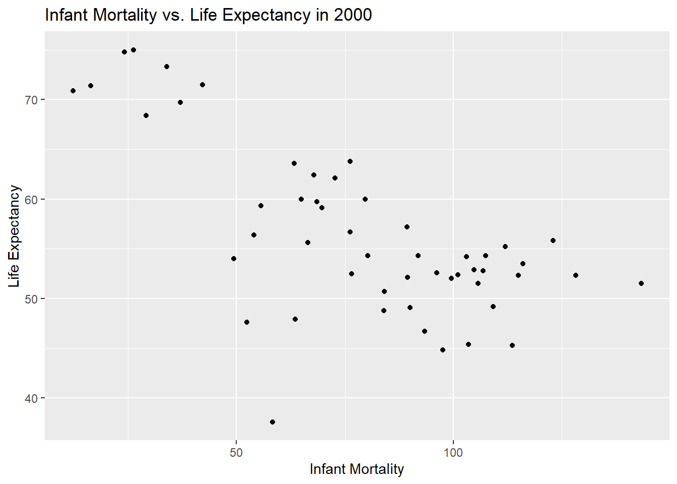
#create a scatterplot of infandlife2ggplot(data=infandlife2, aes(x=infant_mortality, y=life_expectancy))+geom_point()+labs(title="Infant Mortality vs. Life Expectancy in 2000")+xlab("Infant Mortality")+ylab("Life Expectancy")
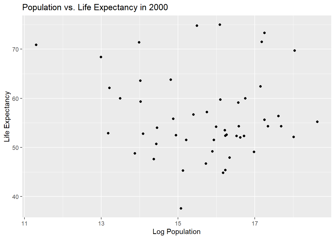
#create a scatterplot of popandlife2ggplot(data=popandlife2, aes(x=log(population), y=life_expectancy))+geom_point()+xlab("Log Population")+ylab("Life Expectancy")+labs(title="Population vs. Life Expectancy in 2000")
##Fit
#fit life expectancy and infant mortalityfit1<-lm(life_expectancy~infant_mortality, infandlife2)#fit life expectancy and populationfit2<-lm(life_expectancy~population, popandlife2)#call summary of fit1summary(fit1)
Call:
lm(formula = life_expectancy ~ infant_mortality, data = infandlife2)

Residuals:
     Min       1Q   Median       3Q      Max
-22.6651  -3.7087   0.9914   4.0408   8.6817

Coefficients:
                 Estimate Std. Error t value Pr(>|t|)
(Intercept)      71.29331    2.42611  29.386  < 2e-16 ***
infant_mortality -0.18916    0.02869  -6.594 2.83e-08 ***
---
Signif. codes:  0 '***' 0.001 '**' 0.01 '*' 0.05 '.' 0.1 ' ' 1

Residual standard error: 6.221 on 49 degrees of freedom
Multiple R-squared:  0.4701,    Adjusted R-squared:  0.4593
F-statistic: 43.48 on 1 and 49 DF,  p-value: 2.826e-08
#call summary of fit2summary(fit2)
Call:
lm(formula = life_expectancy ~ population, data = popandlife2)

Residuals:
    Min      1Q  Median      3Q     Max
-18.429  -4.602  -2.568   3.800  18.802

Coefficients:
             Estimate Std. Error t value Pr(>|t|)
(Intercept) 5.593e+01  1.468e+00  38.097   <2e-16 ***
population  2.756e-08  5.459e-08   0.505    0.616
---
Signif. codes:  0 '***' 0.001 '**' 0.01 '*' 0.05 '.' 0.1 ' ' 1

Residual standard error: 8.524 on 49 degrees of freedom
Multiple R-squared:  0.005176,  Adjusted R-squared:  -0.01513
F-statistic: 0.2549 on 1 and 49 DF,  p-value: 0.6159
Infant mortality and life expectancy are significantly correlated at the 0.05 level but population and life expectancy are not.
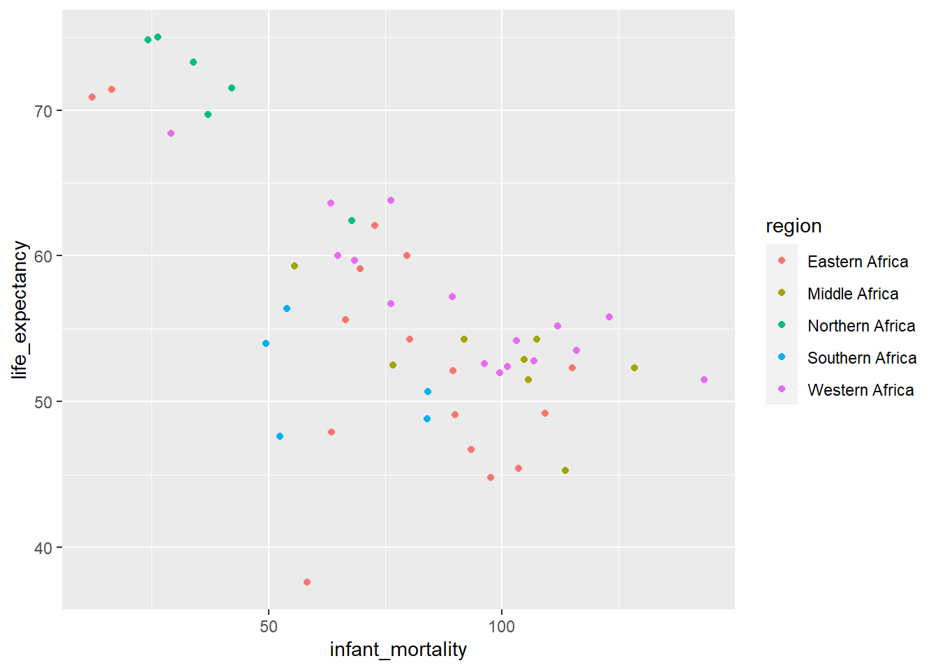
This section is added by Christian Okitondo
Let’s create a plot assessing the relationship between life expectancy and mortality in 2000 and look at the impacted region